Scattergrams - A New Module

Besides porting the EMME/2 system to an always growing range of computer types and graphical equipment, INRO is continuously investing in new developments to make the software package an even more powerful transportation planning tool.

Since the distribution of Release 2.0, a new module has been added to the EMME/2 system. It is called Plot Network Scattergrams and appears as module 2.43 in the menu. As its name indicates, the main goal of this module is to represent link or node data in form of scattergrams, i.e. X-Y diagrams in which the two axes correspond to two arbitrarily chosen link or node attributes and each selected element (node or link) is represented by a graphical symbol appearing on the X/Y point that corresponds to the attribute values of the element.

After having selected the type of scattergram to be plotted (nodes or links), the user is asked to define the attributes to be displayed on the horizontal and the vertical axis. The attributes that may be used are the same as those allowed in expressions of the network calculator (module 2.41). The symbol used for each element, its size and the color in which it is drawn usually default to the value specified in the corresponding module parameters. However, if desired, they may also be varied element by element, in which case a user defined data item is specified, which contains the parameters used for each element. The choice of symbols that may be used corresponds to those used to display demarcations (see section IV-1.41 of the User's Manual for details). The nodes or links to be included in the scattergram are specified in the usual manner, i.e. by using the new link/node select dialog that was presented in the last issue of EMME/2 NEWS. Optionally, a simple linear regression may be performed on the set of points. In this case, the computed regression line is superimposed on the scattergram in the form of a solid center line surrounded by two parallel dotted lines that are spaced upward and downward by one standard deviation. By default, the scattergram is scaled automatically to include all points, but, if desired, the user may redefine horizontal and/&or vertical range manually.

Once the plot has appeared on the screen, the user may use the "c" graphic command to enter into a query mode. Using the graphic cursor, points on the scattergram may be inspected or acted upon individually or in groups, the latter by means of encircling points by closed polygons. Three actions are possible:

• Inspection or Counting: The identifier of the pointed element (node or link) is displayed on the right hand margin. In the case of a group of points surrounded by a polygon, the number of included elements is given.
• Excluding elements: The identifier of the pointed element (or a count for a group of points) is displayed and the element(s) is (are) taken out of the current subset. This may be useful to eliminate "outlyers" before repeating the analysis.
• Marking elements: This option is available when enabled by entering "yes" for the corresponding module parameter and after having specified one of the user defined data items to receive the marking. The identifier of the pointed element (or a count for a group of points) is displayed and the value of the user defined data item of the element(s) is (are) replaced by the current marking value. The marking value may be changed interactively during the query and marking process. The marking operation is extremely useful when some of the elements displayed on the scattergram are subject to other analysis in different modules, since the so marked elements may later be isolated by using the new link/node select dialog.

The interactive commands are based on single characters that are entered after having positioned the graphic cursor at the desired location. The following is a summary of the available commands:

Simple actions:

<space>:             Identify the pointed element

X:                   Exclude the pointed element from the current subset

M:                   Mark the pointed element

Group action commands:

P<space>...<space>C: A closed polygon of arbitrary shape is defined with
                     cursor locations.  The polygon is drawn as the points
                     are entered.  When the final "C" is entered, the
                     polygon is closed and a count of the elements inside
                     the outlined region is displayed on the right hand
                     margin.

O<space>...<space>C: Same as above, but the elements outside the outlined
                     region are counted.

P<space>...<space>X: A polygonal region of the scattergram is defined as
                     above, but the elements inside are excluded from the
                     current subset.

O<space>...<space>X: Same as above, but the elements outside the outlined
                     region are excluded.

P<space>...<space>M: The elements inside the defined region are marked
                     with the current marking value.

O<space>...<space>M: The elements outside the defined region are marked
                     with the current marking value.

Other commands:

G:                   Return to graphic command level.

Q:                   Quit.

R:                   Restart.

U:                   Update plot.

V:                   The user is prompted to enter a new marking value
                     on the right hand margin.

W:                   Redefine horizontal and vertical range and replot
                     scattergram.

This module provides a very general tool for analyzing the network data and it is, of course, impossible to enumerate all its potential uses. Let us just mention a few interesting applications of this module:

a)

Analyze observed vs. predicted volumes and times for calibration purposes.

b)

Calibrate BPR type volume-delay functions from observed link times and volumes, using the network calculator and the linear regression built into this module. This may be done by first transforming the observed times using an expression of the form LN(OBSTIM - 60 * LENGTH / FREEFLOWSPEED), and displaying them against the logarithm of the normalized volumes, i.e. LN(VOLOBS/LANES). So transformed, BPR type volume delay functions become straight lines on the scattergram and the parameters found by the linear regression can easily be transformed back to to the estimated capacity per lane and the exponent that appear in the BPR function.

c)

Analyze convergence of the auto assignment algorithm. This can be done by copying the auto times and volumes obtained after N iterations into, say, UL1 and UL2 (using module 2.41). Then do one more iteration on the same assignment and display the scattergram comparing the volumes (and/ or times) between iteration N and N+1. See the example given below.

This new module is currently in beta test and will be shipped with all new systems delivered after June 1st, 1987. Existing systems will get this new modules along with the next software update, which is scheduled for September.

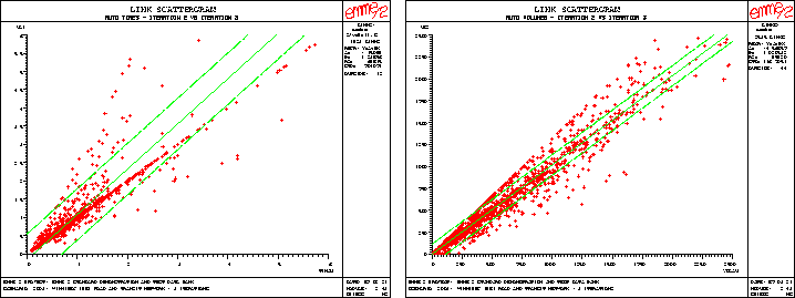
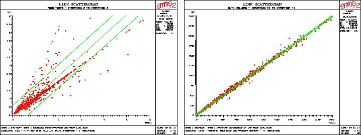
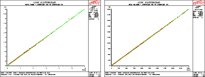
The following is an example of scattergrams generated with module 2.43. It shows the the convergence of the car assignment after different numbers of iterations. The scattergrams compare the auto volumes and auto times on all auto links (mode=c) between two successive iterations, in this case 2 and 3, 10 and 11, and finally, 100 and 101. (It is interesting to note that the 100 iterations of the assignment were performed in less than two hours elapsed time, using the new DSI-780 co-processor.)