(contributed by Heinz Spiess, EMME/2 Support Center)
In most transportation planning applications, the input data which is the most difficult and expensive to obtain is the origin-destination demand matrix. Since the demand data cannot be observed directly, it must be collected by carrying out elaborate and expensive surveys, involving home- or road-based interviews or complicated number plate tagging schemes. By contrast, observed link volumes can be obtained easily and with reasonable precision by simply counting the traffic at certain count post links, either manually or automatically, using mechanical or inductive counting devices.
Thus, it is not surprising that a considerable amount of research has been carried out to investigate the possibility of estimating or improving an origin-destination demand matrix with observed volumes on the links of the considered network. While the models proposed in the past differ greatly in their mathematical formulation and interpretation, they all share the fact that using them for real size networks is difficult, if not impossible. This is due to the complexity of the computations that are involved and the need for very specialized software to carry them out.
During the last two years, we have developed a new approach for the matrix adjustment problem. It is based on the gradient method: While minimizing an objective function based on the difference of observed - predicted volumes on the count post links, the concept of steepest descent, which is inherent to the gradient approach, ensures that the initial demand matrix is not changed more than necessary. The mathematical details of this new method are described in a separate publication (Spiess H., A Gradient Approach for the O-D Matrix Adjustment Problem, CRT Publication #693).
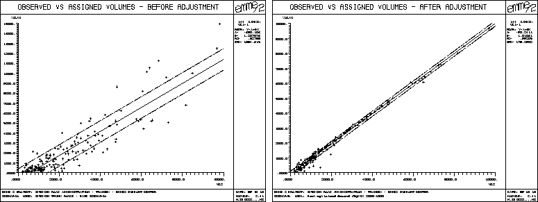
Most important from the practical point of view, is the fact that this method can be implemented as a macro in EMME/2 without the need of any additional software! This also implies that the method can be applied to any network and matrix size that can be handled in EMME/2. The implementation of one iteration of the adjustment method consists in a normal auto assignment, two Additional Options auto assignments, as well as several with network and matrix calculations. A scattergram of the observed vs. assigned volumes on the count post links is generated for each iteration; this facilitates monitoring the progress of the adjustment process.
During 1988 and 1989, we had the opportunity to test the proposed
gradient method and apply it in practice in several studies. The test example
used was based on the standard EMME/2 Winnipeg Demonstration Database. The
applications include two urban applications for the cities of Bern and Basel
(in collaboration with Rapp AG) and the two national road networks of Sweden
(with Transek AB) and Finland (with Finnmap OY)
The table below
gives some characteristics of these applications: number of traffic zones,
number of network links, number of links with observed volumes, the
![]() -value between observed and assigned volumes using the initial
demand, the
-value between observed and assigned volumes using the initial
demand, the ![]() -value after the adjustment, and, finally, the number
of gradient iterations that were carried out for the adjustment.
-value after the adjustment, and, finally, the number
of gradient iterations that were carried out for the adjustment.
| Study | Zones | Links | Counts | initial | final | Iter. |
| Winnipeg | 154 | 2983 | 70 | 0.834 | 0.971 | 11 |
| Basel | 330 | 220 | 229 | 0.923 | 0.970 | 6 |
| Bern | 226 | 2676 | 338 | 0.960 | 0.995 | 20 |
| Sweden | 522 | 3879 | 334 | 0.827 | 0.992 | 20 |
| Finland | 469 | 12476 | 5759 | 0.491 | 0.886 | 30 |
As an example, the scattergrams of observed versus assigned volumes before and after 20 iterations of the adjustment procedure are shown below for the Swedish national road network application. The computations were carried out on a SUN SPARCstation 1 computer. On this equipment, each iteration of the gradient method took about 25 minutes of computing time.

In all applications that were carried out so far, the gradient method was found to perform very well. However, there are some important practical points to consider before applying the algorithm:
The macro DEMADJ is called in the following way:
~<demadj gqp dpq iter relgap normgap gstep [cnt]
The parameter are defined as follows:
Besides the explicit parameters, the DEMADJ macro assumes some implicit
requirements on the data base. The following link user data items and
scalar matrices are used by the macro:
ul1
ul3
ms90
ms91-ms94
Even though only fixed demand assignments are carried out,
it is also recommended that the DEMADJ macro is used with the variable demand
version of the auto assignment (see also the section Bugs+Fixes in this issue).
In addition to the above, the macro itself
contains more detailed instructions in the initial comment section, which
should be read and observed carefully.