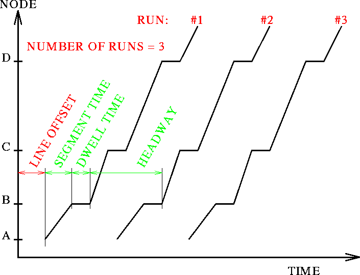
This diagram illustrates how existing and new data items are used to build up the complete time table information for a transit line.
During the past year the most important project aimed at extending EMME/2's modeling capabilities was certainly the development of the Deterministic Transit Assignment. This project is now well into its testing phase and its final version will become part of the upcoming Release 9. Until then, the development may still undergo minor changes regarding the details of the output formats and the user interaction, so it is still a bit too early to announce this development in all its technical details. Nevertheless, this might be a good opportunity to introduce you to the general principles behind this new type of assignment and the basic concepts of its implementation.
Before looking at this new development, let us briefly review the characteristics of EMME/2's standard (stochastic) transit assignment. Being based on the concept of optimal strategies, its main goal is to forecast a transit rider's route choice under steady state assumptions, using only a minimum of input data (i.e. travel times and headways) regarding the operational characteristics of the transit lines. In particular, the standard transit assignment does not consider an explicit time table, but is based only on average vehicle headways and assumes, strictly speaking, an exponential distribution of inter-vehicle times. This type of model is well suited for most urban planning situations, since it performs quite well, but avoids the need of detailed knowledge regarding the exact time table and also of the desired departure or arrival time of each traveler (which is not possible under steady state assumption anyway). While the time table is usually known very well for the base year, producing this level of detail for future year scenarios is practically impossible in most cases.
However, there are certain applications (usually characterized by irregular services, low frequencies and/or long distance) for which the standard transit assignment is less suited. For these applications, we have developed the deterministic transit assignment which is based on complete timetable information. Even before looking at any implementational details, there are some fundamental consequences which such a new type of assignment implies on the demand side:
This being said, let us now look at the basic concepts regarding
the implementation of the deterministic transit assignment.
From a data structure point of view, the most important
requirement is the need to store complete timetable
information. Fortunately, all the time related operational
characteristics which are already in EMME/2 can be
used directly in the time table specification. These are:
| Headways: | Time between two consecutive runs of the same line |
| Segment times: | Running times on transit segments |
| Dwell times: | Passenger exchange times at nodes |
| Line offset: | Departure time of the first run of the line at the initial node of the itinerary, specified in minutes after the beginning of the assignment period. |
| Number of runs: | Number of consecutive vehicle runs (regularly spaced by the line's headway) for which this line operates. As a special case, a value of 0 is used to indicate continuous service. |

This diagram illustrates how existing and new data items are used to
build up the complete time table information for a transit line.
Even if the new development requires only small changes to the existing EMME/2 transit network data structure, it is important to note that, depending on the type of application, it may actually change the meaning of the term transit line. In the extreme case, i.e. when the vehicle runs are not equally spaced or when run-specific assigned volumes are needed, each run will need to be coded as its own transit line.
The second new input data element needed is the specification of the desired departure or arrival time for each trip. For this, a special notation has been developed which offers the following features:
arr=17h45'')The assignment algorithm itself is based on the notion of events. An event is defined as the arrival or departure at a given location (transit segment or node) and a given time. Transitions between two events are denoted as activities and can be classified by the type of the two successive events as shown at the right.
| From-event: | To-event: | Activity: |
| node | node | walk |
| node | segment | wait/board |
| segment | segment | ride |
| segment | node | alight |
In addition to the timetable information itself, the following assignment parameters are used to fine tune the actual route choice:
The deterministic transit assignment produces the following results:
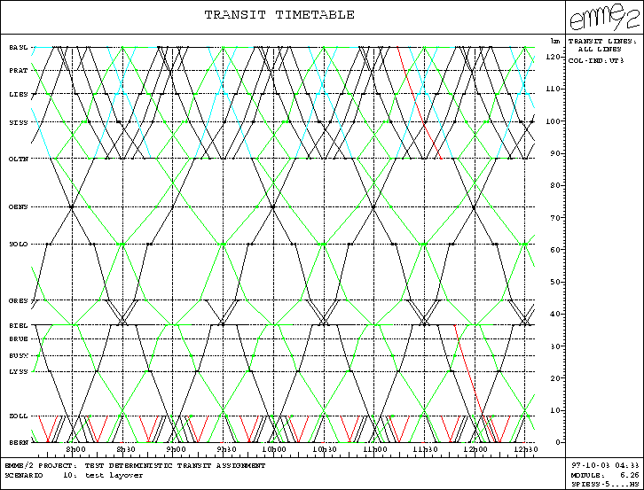
The following example is based on the Swiss intercity railway network. First, an example of a graphical timetable is shown. The vertical axis shows the nodes along the path Bern-Biel-Olten-Basel, whereas the horizontal axis represents the time of day. All trains running on these tracks (in both directions) during the selected time periods are plotted as space-time trajectories.

The following is an excerpt from an assignment report which shows
the optimal itineraries of a trip from Lyss (lyss) to Sissach
(siss) with a desired departure time of 8h00
and the return trip with a desired arrival time of 12h00
(both with an accepted earliness or lateness of 15 minutes):
9.19.1pt
from   1115/lyss   to   1102/siss   desired departure:08h00-15+15                trips:     3

   at         arr    dep  with       --time(late   1.00)--    --cost(late   1.00)--   -distance-
 node        time   time  line/mode  aux  wait   inv cumul    aux  wait   inv cumul   (km) cumul
 1115/lyss         08h04       a   10.00             10.00  15.00             16.00    .50   .50
  115/LYSS  08h14  08h15  S2208           1.00  8.00 19.00         2.50  9.60 28.10  14.44 14.94
  107/BIEL  08h23  08h27  S1413           4.00 46.00 69.00         5.50 55.20 88.80  51.77 66.71
  103/OLTN  09h13  09h17  S2510           4.00 14.00 87.00         5.50 16.80 111.1  11.38 78.09
  102/SISS  09h31  09h31       a   10.00             97.00  15.00             126.1    .50 78.59
 1102/siss  09h41           total: 20.00  9.00 68.00 97.00  30.00 13.50 81.60 126.1        78.59

from   1102/siss   to   1115/lyss   desired arrival:12h00-15+15                trips:     3

   at         arr    dep  with       --time(early   .00)--    --cost(early   .00)--   -distance-
 node        time   time  line/mode  aux  wait   inv cumul    aux  wait   inv cumul   (km) cumul
 1102/siss         10h17       a   10.00             10.00  15.00             15.00    .50   .50
  102/SISS  10h27  10h28  S2521           1.00 15.00 26.00         2.50 18.00 35.50  11.38 11.88
  103/OLTN  10h43  10h47  S1416           4.00 46.00 76.00         5.50 55.20 96.20  51.77 63.65
  107/BIEL  11h33  11h38  S2221           5.00  8.00 89.00         6.50  9.60 112.3  14.44 78.09
  115/LYSS  11h46  11h46       a   10.00             99.00  15.00             127.3    .50 78.59
 1115/lyss  11h56           total: 20.00 10.00 69.00 99.00  30.00 14.50 82.80 127.3        78.59
With the introduction of the deterministic transit assignment in the next release,EMME/2 users will get access to an exciting new tool which greatly extends EMME/2's functionality as a transit planning tool. While it is certainly not meant as a simple substitute for the standard transit assignment, we are convinced that it will open new modeling possibilities, which are beyond the reach of standard steady state assignments.