Heinz Spiess
EMME/2 Support Center
Haldenstrasse 16, CH-2558 Aegerten, Switzerland
October 1989
(Appendices 1 and 2 added August 1997)
This paper (without the appendices) also appeared in
Transportation Science, Vol 24., No. 2, 1990.
The widely used BPR volume-delay functions have some inherent drawbacks. A set of conditions is developed which a ``well behaved'' volume delay function should satisfy. This leads to the definition of a new class of functions named conical volume-delay functions , due to their geometrical interpretation as hyperbolic conical sections. It is shown that these functions satisfy all conditions set forth and, thus, constitute a viable alternative to the BPR type functions.
A PDF version of this document is also available.
In most traffic assignment methods, the effect of road capacity on travel times is specified by means of volume-delay functions t(v) which used to express the travel time (or cost) on a road link as a function of the traffic volume v. Usually these functions are expressed as the product of the free flow time multiplied by a normalized congestion function f(x)
![]()
where the argument of the delay function is the v/c ratio, c being a measure of the capacity of the road.
Many different types of volume-delay functions have been proposed and used in practice in the past (for a review article see Branston [1]). By far the most widely used volume delay functions are the BPR functions (Bureau of Public Roads [2]), which are defined as
![]()
With higher values of ![]() , the onset of congestion effects becomes
more and more sudden. This can be seen in Figures 1, a and b, which show the
BPR type congestion function
, the onset of congestion effects becomes
more and more sudden. This can be seen in Figures 1, a and b, which show the
BPR type congestion function
![]()
for exponents ![]() =2, 4, 6, 8, 10 and 12. This range of alpha values
is also indicative of the wide range that is used in practice, but note that
the values of
=2, 4, 6, 8, 10 and 12. This range of alpha values
is also indicative of the wide range that is used in practice, but note that
the values of ![]() are usually not restricted to integers.
are usually not restricted to integers.
The simplicity of these BPR functions is certainly one reason for their
wide spread use. It is also very convenient that for any value ![]() we have
we have ![]() , i.e. when traffic volume equals the capacity, the
speed is always half the free flow speed.
, i.e. when traffic volume equals the capacity, the
speed is always half the free flow speed.
Fig. 1. BPR functions for (A) small and (B) large v/c ratios
Unfortunately, these BPR functions also have some inherent drawbacks, especially
when used with high values of ![]() :
:
Are there other types of congestion functions that are not (or are less) subject to the drawbacks of the BPR functions? If yes, how would such a ``designer'' volume-delay function look like? Let us first set forth some conditions these functions need to satisfy:
Conditions 1 to 4 hold, of course, for the BPR function and are stated to ensure compatibility with them. Conditions 5, 6 and 7 are imposed in order to overcome the BPR functions' drawbacks a), b) and c) mentioned above.
At least one class of congestion functions exists indeed, as we will show in the remaining part of this note.
Consider an obtuse three-dimensional cone intersected with the two-dimensional X-Y plane. Figure 2 shows the projection of the cone, as well as one possible resulting hyperbolic section. These hyperbolic cone sections have all the desired properties and constitute the base for the conical congestion functions, as we shall name them.
The name ``hyperbolic congestion functions''
would also be appealing, but it has been used in the past
for functions of the form ![]() , see Branston [1].
Furthermore, this name could lead to confusion
with the transcendental hyperbolic functions
sinh and cosh.
, see Branston [1].
Furthermore, this name could lead to confusion
with the transcendental hyperbolic functions
sinh and cosh.
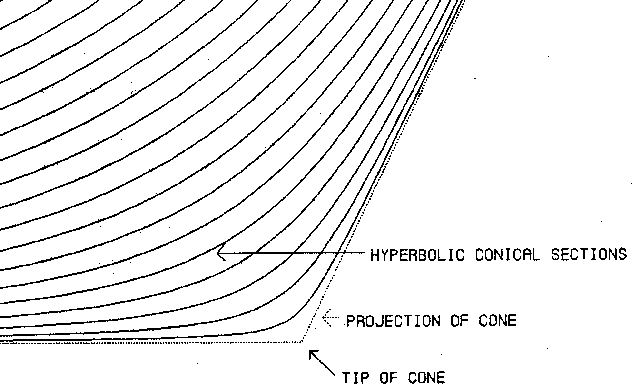 Fig. 2. Hyperbolic conical sections.
Since the mathematical derivation is quite simple but lengthy and only involves basic geometry and elementary algebra, we shall simply state the resulting function and show that it indeed satisfies the conditions 1 to 7 set forth above.
Let the class of conical congestion functions be defined as
![]()
where ![]() is given as
is given as
![]()
and ![]() is any number larger than 1.
is any number larger than 1.
In order to prove that the desired properties hold for ![]() , we need to
evaluate the the first derivative of
, we need to
evaluate the the first derivative of ![]() , which is
, which is
Let us now show, point by point, that the properties 1 to 7 indeed hold for
![]() :
:
Using Pythagoras' theorem, it is easy to see that the second term is
strictly contained between -1 and 1.
Thus ![]() and it follows that
and it follows that ![]() is strictly increasing.
is strictly increasing.
![]()
which, once substituted under the
square root, shows that indeed we have
![]() .
.
![]()
Figure 3, a and b, show the functions ![]() for values of
for values of
![]() =2, 4, 6, 8, 10 and 12. Note the quasi-linear behavior for
x > 1 when comparing Figure 3b to the BPR functions in Figure 1b.
The non-zero gradient of the functions at x=0 can be seen clearly.
=2, 4, 6, 8, 10 and 12. Note the quasi-linear behavior for
x > 1 when comparing Figure 3b to the BPR functions in Figure 1b.
The non-zero gradient of the functions at x=0 can be seen clearly.
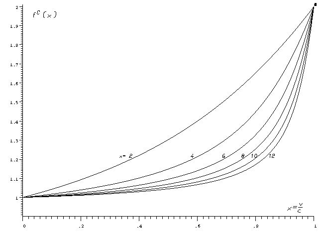
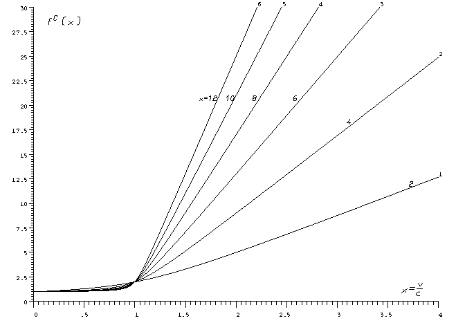 Fig. 3. Conical functions for (A) small and (B) large v/c ratios
We implemented both the BPR and the conical volume-delay function using a little program written in C, in order to compare execution times. The program was compiled and run on the three major families of micro-computers. The results in Table I show that the conical functions can be evaluated more efficiently than the BPR functions, in spite of the apparently more complex formula.
| TABLE I: Computational Efficiency | ||||
| Computer installation | Execution time (msec) | |||
| CPU / FPU | Speed | Compiler | | |
| NSC 32016/32081 | 10Mhz | BSD 4.2 | 1.22 | .98 |
| Intel 80286/80287 | 10Mhz | MS 5.0 | .65 | .37 |
| Motorola 68020/68881 | 17Mhz | SVS | .13 | .09 |
While, to our best knowledge, the class of conical congestion functions proposed here constitutes a new approach, it is interesting to note that a very similar functional form was proposed in an unpublished report prepared in the context of a transportation study for the City of Winnipeg (Traffic Research Corporation [5], Florian and Nguyen [3]). The functions used in that study can also be interpreted as conical sections, but they use more parameters and do not, in general, satisfy the conditions we set forth in the preceding section. For Branston [1] , it was ``doubtful whether these functional form could be of more general user'' and in his article he proceeded to show that these should be approximated by BPR-type functions -- a questionable ``progress'' in the light of our findings.
In a recent transportation study for the City of Basel, Switzerland, the proposed conical volume-delay functions have been used successfully in practice. A dramatic improvement in the convergence of the equilibrium assignment was observed when switching from the previously used BPR functions to the corresponding conical functions, with no practically significant changes in the resulting network flows. This study was carried out using the EMME/2 transportation planning software (Spiess [4]).
In trying to overcome the known disadvantages of the BPR functions,
we have developed a new class of volume-delay functions, the
conical
functions. The interpretation of the parameters used to characterize
the specific congestion behavior of a road link, i.e. capacity
c and steepness ![]() ,
is the same for both BPR and conical function, which makes the transition
to conical functions particularly simple. Since the difference between
a BPR function and a conical function with the same parameter
,
is the same for both BPR and conical function, which makes the transition
to conical functions particularly simple. Since the difference between
a BPR function and a conical function with the same parameter ![]() is
very small within the feasible domain, i.e. v/c <1, the BPR parameters can
be transferred directly in most cases.
is
very small within the feasible domain, i.e. v/c <1, the BPR parameters can
be transferred directly in most cases.
Further research would be needed to develop statistical methods for directly estimating the parameters of the conical functions, using observed speeds and volumes.
(Added August 1997)
When performing system optimum assignments according to Wardrop's first principle, it is necessary to compute the corresponding marginal cost functions. For a given volume-delay function t(v) the corresponding marginal cost function is defined as
![]()
The marginal cost includes on top of the cost perceived by the traveler himself t(v) also the increase in cost t'(v) his traveling causes to for all other v travelers on the same link.
For the BPR function
![]()
the marginal cost is simply
![]()
For the conical function
the marginal cost can be computed using the first derivate
as
After some rearrangements, the above functions can be simplified to
The conical volume-delay functions used in practice include sometimes shifts along the volume axis (e.g. to represent a fixed precharged volume) and also along the time axes (e.g. to use saturated vs free flow time ratios other than 2). These variations are represented by the more general formulation
In the above formula ![]() represents a arbitrary shift along the time axis,
which for standard conical functions corresponds to
represents a arbitrary shift along the time axis,
which for standard conical functions corresponds to ![]() . The coefficient
s, which is 1 for standard conical functions, can be reduced to
. The coefficient
s, which is 1 for standard conical functions, can be reduced to ![]() ,
if a part of the link capacity is taken up by a fixed precharge volume
,
if a part of the link capacity is taken up by a fixed precharge volume ![]() that is not included in the objective function of the system optimum assignment.
that is not included in the objective function of the system optimum assignment.
In this more general case, the marginal cost functions can be written as
(Added August 1997)
As conical volume-delay functions are often used with the
EMME/2 transportation planning software (Spiess [4]),
it might be useful to show how such functions can be efficiently
implemented as EMME/2 function expressions making use, in particular,
of the intrinsic functions put() and get() to optimize
the evaluation of repeated subexpressions.
The standard formulation (12) for the conical volume-delay function can be implemented in a very general way with the following EMME/2 function definition
| fdn | = | |
| +sqrt(get(3)*get(3)+get(2)*get(2))) |
where the function number n, the free flow time
![]() and the function parameter
and the function parameter ![]() have to be replaced by the
corresponding sub-expressions.
have to be replaced by the
corresponding sub-expressions.
If, as is most often the case, ![]() is defined as a constant value,
there is no need to compute the values derived from
is defined as a constant value,
there is no need to compute the values derived from ![]() (such as
(such as ![]() ,
, ![]() and
and ![]() ) each time the function is evaluated. Rather, these
values can be computed once ahead of time, so that the corresponding
values are inserted directly as constants into the function definition.
This allows the following, much more efficient function implementation:
) each time the function is evaluated. Rather, these
values can be computed once ahead of time, so that the corresponding
values are inserted directly as constants into the function definition.
This allows the following, much more efficient function implementation:
| fdn | = | |
If the volume-delay function is to take into account a given fixed precharged
volume (e.g. to represent transit vehicles running on the same link), the
term volau in the above formulae must simply be replaced by the sum
of the auto volumes and the precharged volumes, e.g. assuming that the
precharged fixed volumes are stored in the attribute ul1, then
volau would have to be replaced by (volau+ul1).
For performing a system optimum assignment with EMME/2, the standard
volume-delay functions ![]() must be replaced by the corresponding
marginal cost functions
must be replaced by the corresponding
marginal cost functions ![]() . The following function definition
corresponds to formula (15) for the marginal cost function
. The following function definition
corresponds to formula (15) for the marginal cost function ![]() :
:
| fdn | = | |
| -put((get(1)-0.5)/(get(1)-1)) | ||
| +(get(3)*put(get(1)*(1-get(2)))+put(get(4)*get(4))) | ||
| /sqrt(get(5)*get(5)+get(6))) |
Again, if the function parameter ![]() is a constant, the function
expression can be substantially simplified by computing
is a constant, the function
expression can be substantially simplified by computing ![]() ,
, ![]() and
and ![]() once ahead of time and then inserting the resulting constants
directly into the expression. This lead to the following more efficient
implementation for the marginal cost function
once ahead of time and then inserting the resulting constants
directly into the expression. This lead to the following more efficient
implementation for the marginal cost function ![]() :
:
| fdn | = | |
| +(get(2)*put( |
If the volume-delay function is specified with precharged volumes ![]() , the
formulation of the marginal cost function depend on whether the total
travel cost of the precharged vehicles is considered a part of the
system optimum objective function or not.
, the
formulation of the marginal cost function depend on whether the total
travel cost of the precharged vehicles is considered a part of the
system optimum objective function or not.
In the first case, the marginal cost also includes the increase in travel cost for the precharged vehicles. i.e. we have
![]()
As this case corresponds to a simple shift along the volume axis, the above
formulae remain still valid, one has simply to replace volau
by (volau+ul1) (assuming again the precharged volumes ![]() are
stored in
are
stored in ul1).
However, if the increase in travel costs for the precharged vehicles is not to be considered in the marginal cost function, i.e.
![]()
then we must use ![]() in the general formulation (17).
This leads to the following EMME/2 implementation of the marginal
costs
in the general formulation (17).
This leads to the following EMME/2 implementation of the marginal
costs ![]() for general values of
for general values of ![]() :
:
| fdn | = | |
| -put((get(1)-0.5)/(get(1)-1)) | ||
| +(get(3)*put(get(1)*get(2))+put(get(4)*get(4))) | ||
| /sqrt(get(5)*get(5)+get(6))) |
Finally, for constant values of ![]() , the following implementation
is more efficient, since it avoids the evaluation of constant
sub-expressions for
, the following implementation
is more efficient, since it avoids the evaluation of constant
sub-expressions for ![]() ,
, ![]() and
and ![]() :
:
| fdn | = | |
| +(get(2)*put( |